An overview of classifier-free guidance for diffusion models

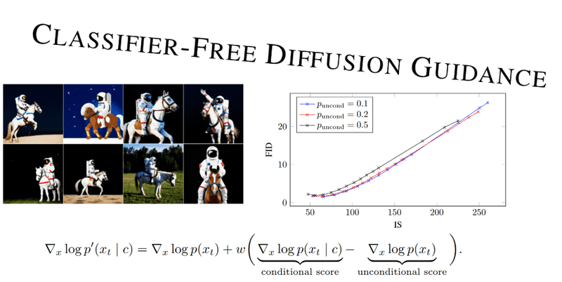
This blog post presents an overview of classifier-free guidance (CFG) and recent advancements in CFG based on noise-dependent sampling schedules. The follow-up blog post will focus on new approaches that replace the unconditional model. As a small recap bonus, the appendix briefly introduces the role of attention and self-attention on Unets in the context of generative models. Visit our previous articles on self-attention and diffusion models for more introductory content on diffusion models and self-attention.

Introduction

Classifier-free guidance has received increasing attention lately, as it synthesizes images with highly sophisticated semantics that adhere closely to a condition, like a text prompt. Today, we are taking a deep dive down the rabbit hole of diffusion guidance. It all began when ^{, in 2021, were looking for a way to trade off diversity for fidelity with diffusion models, a feature missing from the literature thus far. GANs had a straightforward way to accomplish this tradeoff, the so-called truncation trick, where the latent vector is sampled from a truncated normal distribution, yielding only higher likelihood samples in inference.}

The same trick does not work for diffusion models as they rely on the noise to be Gaussian during training and inference. In search of an alternative, ^{came up with the classifier guidance method, where an external classifier model is used to guide the diffusion model during inference. Shortly after, picked up on this idea and found a way of achieving the tradeoff without an explicit classifier, creating the classifier-free guidance (CFG) method. As these two methods lay the groundwork for all diffusion guidance methods that followed, we will spend some time getting a good grasp on these two before exploring the follow-up guidance methods that have developed since. If you feel in need of a refresher on diffusion basics, have a look at , available here.}

Classifier guidance

Narrative: Dhariwal et al. ^{are looking for a way to replicate the effects of the truncation trick for GANs: trading off diversity for image fidelity. They observed that generative models heavily use class labels when conditioned on them. Besides that, they explored other ideas to condition diffusion models on class labels and found an existing method that uses an external classifier $p(c | x)$}

If we had training images without noise, $p(c|x_t)$

where $\nabla_x \log p(c)=0$

Recall that diffusion models generate samples by predicting the score function of the target distribution. The above formula gives us a way of obtaining a conditional score by combining the unconditional and classifier scores. The classifier score is obtained by taking the gradient of the classifier logits w.r.t. the noisy input at timestep $t$. So far, the equation above for the conditional score is not very useful, yet it breaks down the conditional generation into two terms we can control in isolation. Now comes the trick:

where $Z$ is a re-normalizing constant that is typically ignored. We have defined a new guided_score by adding a guidance weight $w$ to the classifier score term. This guidance weight effectively controls the sharpness of the distribution $w \cdot \log p(c \mid x_t)= \log p(c \mid x_t)^w$

Notice I am using the apostrophe $p'(x_t \mid c)$

For $w=1$

However, keep in mind that instead of 2 dimensions, images have height $\times$ width $\times$ three dimensions! It is not clear a priori that forcing the sampling process to follow the gradient signal of a classifier will improve image fidelity. Experiments, however, quickly confirm that the desired tradeoff occurs for sufficiently large guidance weights ^.

Limitations: In high noise scales, it is unlikely to get a meaningful signal from the noisy image, and taking the gradient of the noisy image $p(c \mid x_t)$

Classifier-free guidance

Narrative: The aim of classifier-free guidance is simple: To achieve an analogous tradeoff as classifier guidance does, without the need to train an external classifier. This is achieved by employing a formula inspired by applying the Bayes rule to the classifier guidance equation. While there are no theoretical or experimental guarantees that this works, it often achieves a similar tradeoff as classifier guidance in practice.

TL;DR: A diffusion sampling method that randomly drops the condition during training and linearly combines the condition and unconditional output during sampling at each timestep, typically by extrapolation.

The first step is to solve the guidance equation:

for the explicit conditioning term:

The conditioning term is thus a linear function of the conditional and unconditional scores. Crucially, both scores can be taken from diffusion model training. This avoids training a classifier on noisy images, yet it creates another problem: we now have to train 2 diffusion models: conditional and unconditional. To get around this, the authors propose the simplest possible thing: train a conditional diffusion model $p(x|c)$, with conditioning dropout. During the training of the diffusion model, we ignore the condition $c$ with some probability $p_{\text{uncond}}$

In our new-old formula from classifier guidance:

In this formulation, $\nabla_x \log p(x_t \mid c) – \nabla_x \log p(x_t)$

Same as in classifier-based guidance, CFG leads to “easy to classify”, but often at significant cost to diversity (by sharpening $p_t(c \mid x)^w, w>1$

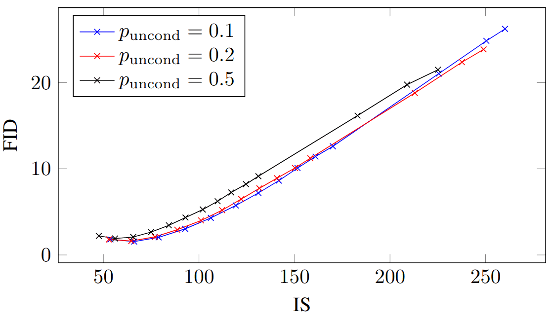
IS/FID curves over guidance strengths for ImageNet 64×64 models. Each curve represents a model with unconditional training probability $p_{\text{uncond}}$

Interleaved linear correction: An essential aspect of CFG is that it’s a linear operation in the high-dimensional image space, applied iteratively in each time step $t$. CFG is interleaved with a non-linear operation, the diffusion model (i.e. a Unet). So, one magical aspect is that we apply a linear operation on the timestep, but it has a profound non-linear effect on the generated image. From this perspective, all guidance methods try to linearly correct the denoised image at the current timestep, ideally repairing visual inconsistencies, such as a dog with a single eye.

Fun fact: The CFG paper was initially submitted and rejected in ICLR 2022 by the title Unconditional Diffusion Guidance. Here is what the AC comments:

“However, the reviewers do not consider the modification to be that significant in practice, as it still requires label guidance and also increases the computational complexity.”

Limitations of CFG

There are three main concerns with CFG: a) intensity oversaturation, b) out-of-distribution samples for very large weights and likely unrealistic images, and c) limited diversity from easy-to-generate samples like simplistic backgrounds. In ^{, the authors discover that CFG with separately trained conditional and unconditional models does not always work as expected. So, there is still much to understand about its intricacies.}

An alternative formulation of CFG

Some papers use a different but mathematically identical formulation CFG. To see that they describe the same equation, here is the derivation ($w = \gamma + 1$

The guidance term is the same as above; the only difference is the weight $\gamma = w – 1$

Static and dynamic thresholding for CFG

Narrative: Static and dynamic thresholding is a simple and naive intensity-based solution to the issues arising from CFG, like oversaturated images.

TL;DR: A linear rescaling on the intensities of the denoised image during CFG-based sampling, either without clipping (static) or with clipping (dynamic) the intensity range.

A large CFG guidance weight improves image-condition alignment but damages image fidelity ^{. High guidance weights tend to produce highly saturated. The authors find this is due to a training-sampling mismatch from high guidance weights. Image generative models like GANs and diffusion models take an image in the range of integers [0,255] and normalize it to [-1,1]. The authors empirically find that high guidance weights cause the denoised image to exceed these bounds since we only drop the condition with some probability during training. This means that the diffusion model is trained conditionally or unconditionally during training. CFG is applied iteratively for all timesteps, leading to unnatural images, mainly characterized by high saturation.}

Static thresholding refers to rescaling the intensity values of the denoised image back to [-1,1] after each step. Nonetheless, static thresholding still partially mitigates the problem and is less effective for large weights. Dynamic thresholding introduces a timestep-dependent hyperparameter $s>1$

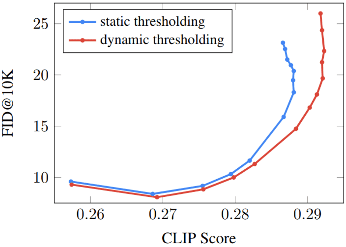
Pareto curves that illustrate the impact of thresholding by sweeping over w=[1, 1.25, 1.5, 1.75, 2, 3, 4, 5, 6, 7, 8, 9, 10]. The figure is taken from ImageGen ^{. No changes were made.}

The authors adaptively decide the value of $s$ for each timestep to be the intensity percentile $p=99.5\%$

Static vs. dynamic thresholding on non-cherry picked 256 × 256 samples using a guidance weight of 5, using the same random seed. The text prompt used for these samples is “A photo of an astronaut riding a horse.” When using high guidance weights, static thresholding often leads to oversaturated samples, while dynamic thresholding yields more natural-looking images. The snapshot is taken from the appendix of the ImageGen paper ^{. CLIP score is a measure of image-text similarity used for text-to-image models. The CLIP score measures the similarity between the generated image and the input text prompt. No changes were made.}

Improving CFG with noise-dependent sampling schedules

Condition-annealing diffusion sampler (CADS)

Narrative: Sadat et al. ^{was one of the first papers to explore non-constant weights in CFG. They noticed that even a simple linear schedule that interpolates between unconditional and conditional generation increases diversity. They saw additional improvements by adjusting the strength of the condition rather than the weight itself.}

TL;DR: A diffusion sampling variation of CFG that adds noise in the conditioning signal, targeting to increase diversity. The noise is linearly decreased during sampling; inversely, the conditioning signal is annealed.

Dynamic CFG baseline

In ^{, the authors create a CFG-based baseline by making the guidance weight dependent on the noise scale $\sigma$. Noise-dependent is equivalent to time-dependent and is used interchangeably. At the beginning of the sampling process, we have $\sigma \rightarrow \sigma_{\text{max}}$}

where $\hat{w}(\sigma)= \alpha(\sigma) w$

The authors provide preliminary results using the so-called Dynamic CFG, which show a decrease in FID.

CADS

First, CADS is a modification of CFG and not a standalone method. CADS employs an annealing strategy on the condition $c$. It gradually reduces the amount of corruption as the inference progresses. More specifically, similar to the forward process of diffusion models, the condition is corrupted by adding Gaussian noise based on the initial noise scale $s$

The schedule is the same as the previous baseline following the pattern: fully corrupted condition (gaussian noise) $\rightarrow$ partially corrupted condition (increasing linearly) $\rightarrow$ uncorrupted conditional.

Rescaling the conditioning signal Adding noise alters the mean and standard deviation of the conditioning vector. To revert this effect, the authors rescale the conditioning vector such that:

where $\psi$ is another hyperparameter $\in (0,1)$

In summary, CADS modulates $c$ (via noise-dependent Gaussian noise) instead of simply applying a schedule to the guidance scale $w$. Interestingly, the diffusion model has never seen a noisy condition during training, which makes it applicable to any conditionally trained diffusion model.

Limited interval CFG

Narrative: Kynkaanniemi et al. took the idea of weak guidance early and stronger guidance later and distilled it into a simple and elegant method. Unlike concurrent works, they identified that the schedule does not need to increase monotonically. They do not try to modify the condition as in CADS and focus on the guidance weight. Using a toy example, they observe that applying guidance at all noise levels causes the sampling trajectories to drift quite far from the data distribution. This is caused because the unconditional trajectories effectively repel the CFG-guided trajectories, mainly during high noise levels. On the other hand, applying CFG at low noise levels on class-conditional models has small to no effect and can be dropped.

TL;DR: Apply CFG only in the intermediate steps of the denoising procedure, effectively disabling CFG at the beginning and end of sampling, practically setting $\gamma$ to 0 (conditional only denoising).

One of the most simple and powerful ideas has been recently proposed by Kynkaanniemi et al. ^{. The authors show that guidance is harmful during the first sampling steps (high noise levels) and unnecessary toward the last inference steps (low noise levels). They thus identify an intermediate noise interval $\in (\sigma_{\text{low}}, \sigma_{\text{high}}]$}

the authors set $\gamma$ to be noise dependent such that $\gamma = \gamma(\sigma)\geq0$

Quantitative results on ImageNet-512. Limiting the CFG to an interval improves both FID and $FD_{\text{DINOv2}}$

Intriguingly, the hyperparameter choice varies based on the metric used to quantify image fidelity and diversity. $FD_{\text{DINOv2}}$

FID and $FD_{\text{DINOv2}}$

Analysis of Classifier-Free Guidance Weight Schedulers

TL;DR: Another concurrent experimental study centered around text-to-image diffusion models was conducted by Wang et al.^{. They demonstrate that CFG-based guidance at the beginning of the denoising process is harmful, corroborating with . Instead of disabling guidance, Wang et al. use monotonically increasing guidance schedules based on a large-scale ablation study. Linearly increasing the guidance scale often improves the results over a fixed guidance value on text-to-image models without any computational overhead.}

There are probably nuanced differences in how guidance works in class-conditional and text-to-image models, so insights do not always translate to one another. While ^{apply the guidance in a fixed interval for text-to-image models and use a simple linear schedule, it’s hard to deduce the best approach. We highlight that a monotonical schedule requires less hyperparameter search and seems easier to adopt for future practitioners in this space. While both works compare with vanilla CFG, the real test would be a human evaluation using all three methods and various state-of-the-art diffusion models.}

Rethinking the Spatial Inconsistency in Classifier-Free Diffusion Guidance

Narrative: Previous works applied noise-dependent guidance scales to improve diversity and the overall visual quality of the distribution of the produced samples. This work focused on improving spatial inconsistencies within an image for text-to-image diffusion models like Stable Diffusion. It is argued that spatial inconsistencies in text-to-image models come from applying the same guidance scale to the whole image.

TL;DR Leverage attention maps to get an on-the-fly segmentation map per image to guide CFG differently for each region of the segmentation map. Here, regions correspond to the different tokens in the text prompt. Visit the appendix first to understand self- and cross-attention maps in this context.

Shen et al. ^{argue that a guidance scale for the whole image results in spatial inconsistencies since different regions in the latent image have varying semantic strengths, focused on text-to-image diffusion. The overall premise of this paper is the following:}

1. Find an unsupervised segmentation map (per token in the text prompt) based on the internal representation of self- and cross-attention (see Appendix).

2. Refine the segmentation maps to make the object boundaries clearer and remove internal holes.

3. Use the segmentation maps to scale the guided CFG score to equalize the varying guidance scale per semantic region $W_t \in R^{H_{img} \times W_{img}}$

where $\odot$ is an element-wise product known as Hadamrd product.

To get a segmentation map on the noisy image $x_t$

from the last two layers and heads (from the smallest two resolutions of the Unet encoder) are upsampled and aggregated ($C_t^{agg}$

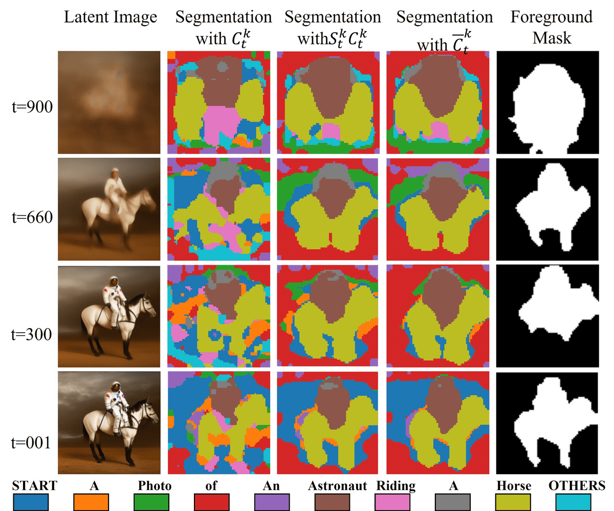
First column: predicted image at timestep $t$. Second column: segmentation map from cross-attention only ($C_t^{agg}$

The result is shown in the fourth column in the above figure . Here, $S_t$

Based on $i_{\max}$

Cross-attention in Unet diffusion models. Visual and textual embedding are fused using cross-attention layers that produce spatial attention maps for each textual token. Critically, keys $K$ and values $V$ come from the condition (text prompt). Snapshot is taken from Hertz et al. ^{. No changes were made.}

How cross-attention works. Previous studies provide intuition on the impact of the attention maps on the model’s output images. To start, here is how the cross-attention operation as it is implemented in Unets at each timestep $t$.

for query $Q_t \in \mathbb{R}^{(h \times w) \times d}$

where $C_t \in \mathbb{R}^{(h \times w) \times d}$

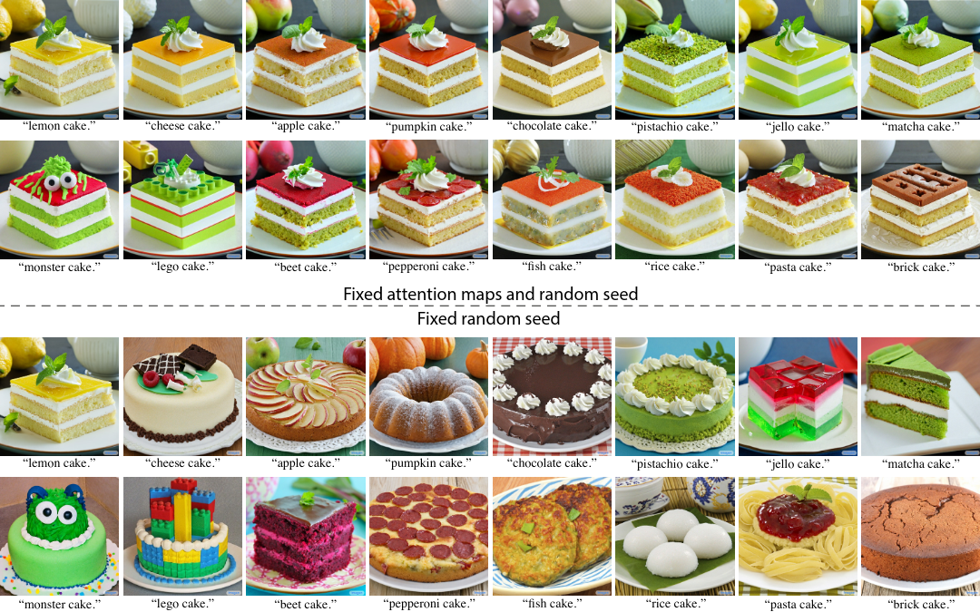
The figure is taken from Hertz et al. ^{. No changes were made.}

Condition swap in cross-attention. In ^{, the authors show the impact of changing the condition during inference for text-to-image models. From left to right in the figure below, the five images are produced with different transition percentages: 0%, 7%, 30%, 60%, and 100%. In the last steps of denoising, the condition has no visual impact. Switching condition after 40% of the denoising overwrites the imprint of the initial condition.}

Visualizing the effect of prompt switching during diffusion sampling. Second column: in the last steps of denoising, the text inputs have negligible visual impact, indicating that the text prompt is not used. Third column: the 70-30 ratio leaves imprints in the image from both prompts. Fourth column: the first 40% of denoising is overridden from the second prompt. The denoiser utilizes prompts differently at each noise scale. The snapshot is taken from ^{, licensed under CC BY 4.0. No changes were made}

Self-attention vs cross-attention. However, the cross-attention module in the Unet should be distinct from the self-attention module. We have identified that the cross-attention module only exists in text-to-image diffusion Unets, while the self-attention component also exists in class conditional and unconditional diffusion models. So even though we tend to represent $c$ with the condition in both cases, class condition, and test prompts are processed differently under the hood. Here is how self-attention is computed in a Unet, for query $Q_t \in \mathbb{R}^{(h \times w) \times d}$

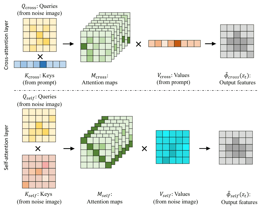
Cross and self-attention layers in Unet denoisers such as Stable Diffusion. The image is taken from ^{, licensed under CC BY 4.0. No changes were made.}

Liu et al. ^{conducted a large-scale experimental analysis on Stable diffusion, focused on image editing. The authors demonstrate that cross-attention maps in Stable Diffusion often contain object attribution information. On the other hand, self-attention maps play a crucial role in preserving the geometric and shape details. The $K,V$ pair comes from the same image during image synthesis and the source/reference image for image editing.}

Conclusion

We have presented an overview of CFG and its schedule-based sampling variants. In short, monotonically increasing schedules are beneficial, especially for text-to-image diffusion models. Alternatively, using CFG only in an intermediate interval reaps all the desired benefits without oversacrificing diversity while keeping the computation budget lower than CFG. Finally, the self and cross-attention modules of diffusion Unets provide useful information that can be leveraged during sampling, as we will see in the next one. The next article will investigate CFG-like approaches that try to replace the unconditional model, in an effort to make CFG a more generalized framework. For a more introductory course, we highly recommend the Image Generation Course from Coursera.

If you want to support us, share this article on your favorite social media or subscribe to our newsletter.

Citation

@article{adaloglou2024cfg,
  title   = "An overview of classifier-free guidance for diffusion models",
  author  = "Adaloglou, Nikolas, Kaiser, Tim",
  journal = "theaisummer.com",
  year    = "2024",
  url     = "https://theaisummer.com/classifier-free-guidance"
}

Disclaimer

Figures and tables shown in this work are provided based on arXiv preprints or published versions when available, with appropriate attribution to the respective works. Where the original works are available under a Creative Commons Attribution (CC BY 4.0) license, the reuse of figures and tables is explicitly permitted with proper attribution. For works without explicit licensing information, permissions have been requested from the authors, and any use falls under fair use consideration, aiming to support academic review and educational purposes. The use of any third-party materials is consistent with scholarly standards of proper citation and acknowledgment of sources.

References

Deep Learning in Production Book 📖

Learn how to build, train, deploy, scale and maintain deep learning models. Understand ML infrastructure and MLOps using hands-on examples.

Learn more

* Disclosure: Please note that some of the links above might be affiliate links, and at no additional cost to you, we will earn a commission if you decide to make a purchase after clicking through.